Xpress-SP Reference Manual

[Previous chapter] [Next chapter]

Illustrative examples

In this chapter, we demonstrate the use of Xpress-SP's modeling and solution techniques in solving stochastic problems from various streams such as supply chain management, finance, energy sector, transportation, and forest planning. A short description of a problem from each sector is given, followed by the model used to solve the problem and its implementation with Mosel.

Farm production planning

In this section, we show how to model a simple 2-stage model using Xpress-SP. We model the farmer's problem (see [BL97a]), where a farmer needs to make decisions regarding the devotion of available land to different products: wheat, corn and sugar beet, during the winter season. The yield is realized in the summer and depends on the overall weather during the year (e.g., bad, ok, good). The farmer must produce a certain amount of products for the cattle feed. Then the farmer must also decide how much of each product needs to be purchased or sold depending on the yield. There is an additional restriction on the selling price of sugar beet because of quota restriction. The model entities are described below.

Sets

Stages: {Winter, Summer}

Products: {Wheat, Corn, Sugar Beet}

Constraints

Minimum production for cattle feed

Quota restriction on sugar beet production

Variables

x_i: acres of land devoted to product i

w_wheat, w_corn: tons of wheat and corn sold respectively

y_wheat, y_corn: tons of wheat and corn purchased respectively

w_favor, w_unfavor: tons of sugar beet sold at favorable and unfavorable price respectively

Model
model farmer
 uses 'mmsp'
 
 parameters
  Explicit=false         ! Explicitly create tree or use the joint 
                         ! distribution feature
 end-parameters
 
 forward procedure Analyse(prob: string) 

 setparam('xsp_scen_based', false)

 declarations
!{"Wheat","Corn","Sugar Beet Favorable","Sugar Beet Unfavorable"}
  AllProducts={"Wht","Crn","SugBtFav","SugBtUnfav"}
  Products={"Wht","Crn","SugBt"}
  WheatAndCorn={"Wht","Crn"}
  
  PlantingCost: array(Products) of real
  SellingPrice: array(AllProducts) of real
  PurchasePrice: array(WheatAndCorn) of real
  MinimumRequirement: array(WheatAndCorn) of real
  TotalAvailableLand: real
  MaxSugarBeetQuota: real
 end-declarations
 
 PlantingCost:= [150,230,260]
 SellingPrice:= [170,150,36,10]
 PurchasePrice:= [238,210]
 MinimumRequirement:= [200,240]
 TotalAvailableLand:= 500
 MaxSugarBeetQuota:= 6000
 
 declarations
  Stages={"Wint","Summ"}
  yield: array(Products) of sprand
  
  x: array(Products) of spvar
  y: array(WheatAndCorn) of spvar
  w: array(AllProducts) of spvar
  
  TotalCost: splinctr
  LandUtilized: splinctr
  MinCattleFeedRequirement: array(WheatAndCorn) of splinctr
  SugarBeetProduction: splinctr
  SugarBeetQuota: splinctr
 end-declarations
 
! Stages
 spsetstages(Stages)
 forall(p in Products) spsetstage(yield(p),"Summ")
 
! Scenarios
 declarations
  S = 3
  Values: array(Products,1..S) of real
 end-declarations

 forall(s in 1..S) prob(s):=1/3
 Values:= [3,2.5,2,
           3.6,3,2.4,
           24,20,16]
 if Explicit then  
  spcreatetree(S)         
  spsetprobcond(2,prob)
  forall(p in Products,s in 1..S)
  spsetrandatnode(yield(p),s,Values(p,s))
  spgentree
 else
  spsetdist(union(p in Products) {yield(p)},Values,prob)
  spgenexhtree
 end-if
 
! Model
 TotalCost:= sum(p in Products) PlantingCost(p)*x(p)-
             sum(p in AllProducts) SellingPrice(p)*w(p)+
             sum(p in WheatAndCorn)PurchasePrice(p)*y(p)
 LandUtilized:= sum(p in Products) x(p) <= TotalAvailableLand
 forall(p in WheatAndCorn)
  MinCattleFeedRequirement(p):= yield(p)*x(p)+y(p)-
                                w(p) >= MinimumRequirement(p)
 SugarBeetProduction:= sum(p in {"SugBtFav","SugBtUnfav"}) 
                        w(p)<=yield("SugBt")*x("SugBt")
 SugarBeetQuota:= w("SugBtFav") <= MaxSugarBeetQuota
 
 forall(p in Products) spsetstage(x(p),"Wint")
 forall(p in WheatAndCorn) spsetstage(y(p),"Summ")
 forall(p in AllProducts) spsetstage(w(p),"Summ")
  
! Analysis
 declarations
  Problem={"Rec","Exp Val","Exp Val wt rec","Perf Inf",
           "Perf Inf wt rec"}
 end-declarations
 forall(problem in Problem) Analyse(problem)

!***************************************************************
 
 procedure Analyse(problem:string)
  write("Solving " + problem + " Problem")

  case problem of
  "Exp Val":         minimize(TotalCost,XSP_EV)
  "Exp Val wt rec":  minimize(TotalCost,XSP_EV+XSP_REC)
  "Perf Inf":        minimize(TotalCost,XSP_PI)
  "Perf Inf wt rec": minimize(TotalCost,XSP_PI+XSP_REC)
  "Rec":             minimize(TotalCost,XSP_REC)
  end-case

  writeln("\n------------------------------------------")
  write("Culture           |")
  forall(p in Products) write(strfmt(p,7))
  writeln("\n------------------------------------------")
  if(problem="Perf Inf") then
   forall(s in 1..spgetscencount) do
    write("Surface (acres) ",s," |");
    forall(p in Products) write(strfmt(getsolinscen(x(p),s),7,2));
    writeln
   end-do
  else 
   write("Surface (acres)   |");
   forall(p in Products) write(strfmt(speval(x(p)),7,2))
   writeln
  end-if
  writeln("TotalProfit=$",-getobjval)
  writeln("------------------------------------------")
  
  case problem of
  "Exp Val wt rec","Perf Inf wt rec":
   do
    forall(p in Products) spunfix(x(p))
    spsethidden(LandUtilized,false)
   end-do
  end-case
  writeln  
 end-procedure
 
 end-model
Results

The overall expected profit is $108,390. The solution, which was obtained considering all circumstances, is ideal. It also allows selling some sugar beet at an unfavorable price or having unused quota and hence hedging against various scenarios. The model also provides the option of either creating the scenario tree explicitly or using the joint distribution functionality in mmsp. The following output is obtained after the model is run in Xpress-SP.
        Solving Rec Problem
 ------------------------------------------
 Culture   |    Wht    Crn  SugBt
 ------------------------------------------
 Surface
 (acres)   | 170.00  80.00 250.00
 TotalProfit=$108390
 ------------------------------------------
 
       Solving Exp Val Problem
 ------------------------------------------
 Culture   |    Wht    Crn  SugBt
 ------------------------------------------
 Surface
 (acres)   | 120.00  80.00 300.00
 TotalProfit=$118600
 ------------------------------------------
 
 mmsp warning 101: fixing variables and hiding constraints
 mmsp warning 102: hiding constraint, since all variables are hidden/fixed
       Solving Exp Val wt rec Problem
 ------------------------------------------
 Culture   |    Wht    Crn  SugBt
 ------------------------------------------
 Surface
 (acres)   | 120.00  80.00 300.00
 TotalProfit=$107240
 ------------------------------------------
 
       Solving
 Perf Inf Problem
 ------------------------------------------
 Culture   |    Wht    Crn  SugBt
 ------------------------------------------
 Surface
 (acres) 1 | 183.33  66.67 250.00
 Surface
 (acres) 2 | 120.00  80.00 300.00
 Surface
 (acres) 3 | 100.00  25.00 375.00
 TotalProfit=$115406
 ------------------------------------------
 
 mmsp warning 101: fixing variables and hiding constraints
 mmsp warning 102: hiding constraint, since all variables are hidden/fixed
       Solving
 Perf Inf wt rec Problem
 ------------------------------------------
 Culture   |    Wht    Crn  SugBt
 ------------------------------------------
 Surface
 (acres)   | 134.44  57.22 308.33
 TotalProfit=$103717
 ------------------------------------------
Finance

Stochastic programming has been extensively studied and applied in various sectors of finance, e.g., asset liability management, portfolio management, financial planning, etc. Here we consider a simple stochastic problem for financial planning [BL97b].

Model description

We currently want to invest $b in stocks and bonds. At the end of T-1 years, we would like to exceed the goal $G. The investment is changed every year. The excess income would imply an income of q% of the excess income and shortage would imply borrowing at r% of the amount short. The plot of the utility function for wealth at the end would look as follows:

Figure 6.1: Utility function

We also assume that at each stage the return on stocks and bonds is 1.25 and 1.14 or 1.06 and 1.12 each with probability 0.5

Decision variables

x_it: amount invested in asset i at time t

y: shortage

w: excess

Constraints

Balance of initial investment, returns and goal meeting requirements

Xpress model
model stochasticStockAndBondModel
 uses 'mmsp'
 parameters
  T=4
  Explicit=true
 end-parameters

 forward procedure generateTree

 declarations
  Assets={"Stocks","Bonds"}
  Stages=1..T
  x: array(Assets,1..T-1) of spvar     ! Amount invested
  w,y: spvar                           ! Shortage, excess
  return: array(Assets,2..T) of sprand ! Return on investment
  b,G: real                            ! Initial wealth, goal(in $1000)
  q,r:                                 ! Excess,shortage(in %)
  ExpectedUtility: splinctr
  Balance: array(1..T) of splinctr
 end-declarations

! Data
 b:=55;G:=80;q:=1;r:=4

 spsetstages(Stages)
 forall(i in Assets,t in 2..T) spsetstage(return(i,t),t)
 generateTree

 forall(i in Assets,t in 1..T-1) spsetstage(x(i,t),t)
 spsetstage(y,T)
 spsetstage(w,T)

 ExpectedUtility:=q*y-r*w
 forall(t in 1..T)
  if t=1 then 
   Balance(t):=sum(i in Assets) x(i,t)=b;
  elif t=T then 
   Balance(t):=sum(i in Assets) return(i,t)*x(i,t-1)- y+w=G;
  else Balance(t):=-sum(i in Assets) x(i,t)+
   sum(i in Assets) return(i,t)*x(i,t-1)=0;
  end-if
  
 setparam("xsp_scen_based",false)
 setparam('xsp_verbose',false)
 maximize(ExpectedUtility)

 ObjvalRP:=getobjval
 writeln("Obj value in recourse problem = ", strfmt(ObjvalRP,0,2))
 forall(t in 1..T-1) spfix(x("Bonds",t),0)

 maximize(ExpectedUtility)
 writeln("Obj value in recourse problem = ", strfmt(getobjval,0,2))
 writeln("VSS (if all investments in Stocks only) = ", strfmt(ObjvalRP-
   getobjval,0,2))
 forall(t in 1..T-1) spunfix(x("Stocks",t))
 
!***********************************************************
 procedure generateTree 
  declarations
   SetSrnd: set of sprand
   val: array(1..2,1..2) of real
   prob: array(1..2) of real
   StockVal,BondVal,BranchProb: array(1..2) of real
  end-declarations
  
  if(Explicit) then 
   spcreatetree(2)          ! Binary tree
   StockVal:=[1.25,1.06]
   BondVal:=[1.14,1.12]
   BranchProb:=[.5,.5]
   forall(t in 2..T) do                    ! Set Srnds
    spsetrand(return("Stocks",t),StockVal)
    spsetrand(return("Bonds",t),BondVal)
   end-do
   spsetprobcond(BranchProb)               ! Set branch probabilities
   spgentree                               ! Generate tree
  else                      ! Use joint distribution functionality
   val:=[1.25, 1.06, 1.14, 1.12]
   prob:=[.5, .5] 
   forall(t in 2..T) do
    SetSrnd:={}
    forall(i in Assets) SetSrnd+={return(i,t)} 
    spsetdist(SetSrnd,val,prob)
   end-do
   spgenexhtree
  end-if
   
 end-procedure

end-model
Note that in the above model, users may implicitly set the stages of return and x by setting the control parameter xsp_implicit_stage to true, but this would also set the variables w and y to the first stage, therefore their stages have to be set explicitly using the function spsetsatage().

Results

The optimal value of expected utility is –1.514. The initial investment in stocks and bonds is $41479 and $13520 respectively. The model also demonstrates how users may fix certain decisions and solve the problem in the stochastic framework. In the above model, the impact of placing all the funds in stocks is evaluated. It is observed that the expected utility using this strategy is -3.79. Other results can be analyzed in IVE.

Figure 6.2: Stocks and bond model in IVE

Energy

Stochastic programming also finds wide-spread application in the energy sector where the demand for power and its prices are constantly changing. It has been used for solving various problems such as capacity expansion, unit commitment, etc. Here, we discuss an implementation of a capacity expansion model using Xpress-SP.

Model description

In a power-generating plant, the trend of yearly power demand looks as follows:

Figure 6.3: Load duration curve

Here, for simplicity, we consider three modes of operations; namely low, average, and high. Clearly, the trend of power demanded in each year may vary depending on various factors such as rainfall, weather conditions, etc. We also consider three technologies (old, current, and new). Capacity expansion plans and the operational decisions need to be laid out for next three years. The objective is to minimize the expected total investment and production cost. The stochastic model entities are described below.

Parameters

Stages = 1,...,4 : indexed by t

Technology = {old,curr,new} :indexed by i

Modes={low,avg,high} :indexed by j

Data

g_it: existing capacity of technology i added at time t

r_it_:investment cost per unit of capacity of technology i added at time t

q_it:production cost per unit of capacity of technology i added at time t

Decision variables

x_it: capacity of technology i added at time t

y_ijt:capacity of type i dedicated in mode j at time t

Constraints

Accumulated Capacity balance

Demand balance

Objective

minimize the expected total investment and production cost

The capacities are added in the first two years and hence the total available capacities are realized in the second and the third year. In the years two through four, the available capacities are distributed among different modes.

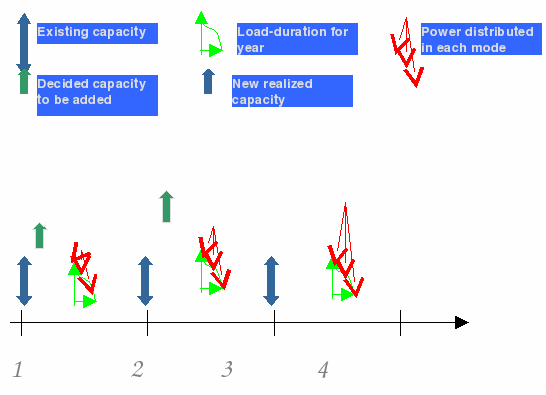
Figure 6.4: Production planning schedule

The scenarios are created by discretizing the load-duration curve. For simplicity, the duration in each mode is considered one-third of a year. We present three ways of generating scenarios:

Exhaustive: The demand (low, average, and high) has an independent distribution in each year.

Stage symmetric: There are 8, 5, and 3 load-duration curves possible in the first, second, and third year respectively.

Explicit: The demand in the subsequent year depends on the earlier years' demand and hence, all possible realizations are explicitly defined.

Exhaustive model
model CapacityExpansion
 uses 'mmsp'
 parameters
  T=4                                  ! Years
 end-parameters

 forward procedure generateExhaustiveTree

 declarations
  Stages=1..T
  Technology={"old","curr","new"}
  Modes={"low","avg","high"}
  
  r: array(Technology,1..T-2) of real   ! Investment cost in $1000/MW cap. added
  g: array(Technology,1..T-1) of real   ! Existing capacity in MW
  q: array(Technology,2..T) of real     ! Unit production cost in $1000/MWh
  tau: real                             ! Time in hour spent in each mode
  Budget: real                          ! Max. additional capacity in MW
  Penalty: real                         ! For not meeting demand in $1000/MW

  d: array(Modes,2..T) of sprand        ! Total demand in MW
  umd: array(Modes,1..T-1) of spvar     ! Total unmet demand in MW
  x: array(Technology,1..T-2) of spvar  ! Additional capacity in MW
  w: array(Technology,2..T-1) of spvar  ! Total available capacity in MW
  y: array(Technology,Modes,2..T) of spvar ! Capacity used in production in MW
  Cost: splinctr
  BudgetSpent: splinctr
  AccumulatedCapacity: array(Technology,2..T-1) of splinctr
  Demand: array(Modes,1..T-1) of splinctr
  Capacity: dynamic array(Technology,1..T-1) of splinctr
 end-declarations
  
! Read in data from external file
 initializations from 'CapacityExpansion.dat'
  r q g tau Budget Penalty
 end-initializations
  
 setparam('xsp_implicit_stage',true)
 spsetstages(Stages)
 generateExhaustiveTree
  
 Cost:= sum(t in 1..T-2,i in Technology) r(i,t)*x(i,t) +
        sum(t in 2..T,i in Technology,j in Modes) q(i,t)*tau*y(i,j,t) +
        sum(j in Modes,t in 1..T-1) Penalty*umd(j,t)
 BudgetSpent:= sum(i in Technology,t in 1..T-2) x(i,t)<=Budget
 forall(i in Technology,t in 2..T-1)
  if (t-1>=2) then 
   AccumulatedCapacity(i,t):= w(i,t)=x(i,t-1)+w(i,t-1);
  else
   AccumulatedCapacity(i,t):= w(i,t)=x(i,t-1)
  end-if
 forall(j in Modes,t in 1..T-1) 
  Demand(j,t):= umd(j,t) + sum(i in Technology) y(i,j,t+1)>=d(j,t+1)
 forall(i in Technology,t in 1..T-1)
  if(t>=2) then 
   Capacity(i,t):=sum(j in Modes) y(i,j,t+1)<=(g(i,t)+w(i,t));
  else
   Capacity(i,t):=sum(j in Modes) y(i,j,t+1)<=g(i,t)
  end-if
  
 forall(t in 2..T) OperatingCost(t):=sum(i in Technology,j in Modes) 
        q(i,t)*tau*y(i,j,t)

 minimize(Cost)
 writeln(getobjval)
 
!************************************************************** 
 procedure generateExhaustiveTree
  declarations
   E=3                      ! Max no. of values, each demand can assume
   val,prob:array(Modes,2..T,1..E) of real
  end-declarations

  initializations from 'CapacityExpansionExhaustive.dat'
   val prob
  end-initializations

  declarations
   vals,probs:array(1..E) of real
  end-declarations
                      
  forall(j in Modes,t in 2..T) do
   forall(e in 1..E) do
    vals(e):=val(j,t,e)
    probs(e):=prob(j,t,e)
   end-do
   spsetdist(d(j,t),vals,probs)
  end-do
  spgenexhtree
 end-procedure
  
 end-model
Data files:

CapacityExpansion.dat:
r:[464,500,
    508,507,
    534,490]
 q:[.040,.034,.032,
    .030,.022,.021,
    .019,.018,.016] 
 g:[80,50,20,
    70,35,20,
    40,25,15]
 
 tau:2900
 Budget:350
 Penalty:1300
CapacityExpansionExhaustive.dat:
val:[20,25,0,
      28,33,0,
      36,40,0,
 
      50,55,0,
      58,63,0,
      66,70,0,
 
      80,85,0,
      88,93,0,
      96,100,0]
! replace zeros by some other numbers to get more possible realizations 
! andscenarios.
       
 prob:[.5,.5,0,
       .5,.5,0,
       .4,.6,0,      
 
       .6,.4,0,
       .4,.6,0,
       .6,.4,0,       
 
       .4,.6,0,
       .5,.5,0,
       .5,.5,0]
Stage symmetric model

In order to generate a scenario tree, which is symmetric with respect to stage, the procedure generateExhaustiveTree in the above example can be replaced by the procedure generateStageSymmetricTree which is defined below. The parameter Dep when set to true, would create the tree using the joint probability distribution facility in mmsp.
 procedure generateStageSymmetricTree
  declarations
   NumBranch:array(2..T) of integer
  end-declarations

  initializations from DIR+"CapacityExpansionStage.dat"
   NumBranch
  end-initializations

  MaxBranch:=max(t in 2..T) NumBranch(t)
  
  declarations
   BranchProb:array(2..T,1..MaxBranch) of real
   BranchValues:array(Modes,2..T,1..MaxBranch) of real
   Prob,Values:array(1..MaxBranch) of real
  end-declarations

  initializations from DIR+"CapacityExpansionStage.dat"
   BranchProb BranchValues
  end-initializations

  declarations
   AllDem:set of sprand
   Val:array(Modes,1..MaxBranch) of real
  end-declarations
   
  if(Dep) then
   forall(t in 2..T) do
    AllDem:=union(j in Modes) {d(j,t)}
    forall(b in 1..MaxBranch) Prob(b):=0
    forall(b in 1..NumBranch(t)) Prob(b):=BranchProb(t,b)
    forall(j in Modes,b in 1..MaxBranch) Val(j,b):=0
    forall(j in Modes,b in 1..NumBranch(t)) Val(j,b):=BranchValues(j,t,b)
    spsetdist(AllDem,Val,Prob)   
   end-do
   spgenexhtree
  else
   spcreatetree(NumBranch)
   forall(t in 2..T) do
    forall(b in 1..NumBranch(t)) Prob(b):=BranchProb(t,b)
    spsetprobcond(t,Prob)
   end-do 
   forall(t in 2..T,j in Modes) do
    forall(b in 1..NumBranch(t)) Values(b):=BranchValues(j,t,b)
    spsetrand(d(j,t),Values)
   end-do
   spgentree 
  end-if 
 end-procedure
CapacityExpansionStage.dat:
 NumBranch:[8,5,3]
 BranchProb:[0.15,0.15,0.1,0.1,0.2,0.1,0.1,.1,
   0.2,0.2,0.2,0.2,0.2,0,0,0,
   .25,.5,.25,0,0,0,0,0]
 BranchValues:[80,81,82,83,84,86,87,88,   
  86,88,90,93,95,0,0,0,   
  96,98,100,0,0,0,0,0,    
  50,51,52,53,54,56,57,58,   
  56,58,60,63,65,0,0,0,   
  66,68,70,0,0,0,0,0,  
  20,21,22,23,24,26,27,28,   
  26,28,30,33,35,0,0,0,
  36,38,40,0,0,0,0,0]
Explicit model

A scenario tree with seven scenarios in the above example can be generated as follows:
 procedure generateExplicitTree
  declarations
   S=7                           ! No. of scenarios
   A:array(1..S,1..T) of integer ! Node numbers in tree
   N:array(1..T) of integer      ! Number of nodes in each stage
  end-declarations
 
  initializations from DIR+'CapacityExpansionExplicit.dat'
   A N
  end-initializations

  spcreatetree(A)
  Nmax:=max(t in 1..T) N(t)

  declarations
   val:array(2..T,Modes,1..Nmax) of real
   prob:array(2..T,1..Nmax) of real
  end-declarations
 
  initializations from DIR+'CapacityExpansionExplicit.dat'
   val prob
  end-initializations
  
  forall(t in 2..T,n in 1..N(t)) spsetprobcondatnode(t,n,prob(t,n))
  forall(t in 2..T,j in Modes,n in 1..N(t))
 
  spsetrandatnode(d(j,t),n,val(t,j,n))
  spgentree
 end-procedure
CapacityExpansionExplicit.dat:
A:[1,1,1,1,
    1,1,2,2,
    1,1,2,3,
    1,1,2,4,
    1,2,3,5,
    1,2,3,6,
    1,3,4,7]
 
 N:[1,3,4,7]
 
 val:[20,25,30,0,0,0,0,
      50,55,60,0,0,0,0,
      30,60,90,0,0,0,0,
      25,35,30,30,0,0,0,
      55,65,60,60,0,0,0,
      85,95,90,90,0,0,0,
      38,35,38,40,36,39,38,
      68,65,68,70,66,69,68,
      98,95,98,100,96,99,98]
 
 prob:[.333,.333,.333,0,0,0,0,
       .5,.5,1,1,0,0,0,
       1,.333,.333,.333,.5,.5,1]
Results

The results for each of these models with respective scenario generation schemes can be obtained using the standard functions available in the mmsp module and IVE. The plot of other entities, e.g., the operating cost in stage 3, can be viewed in IVE (see Figure Operating cost in third stage (scenario generation scheme: exhaustive)).

Figure 6.5: Operating cost in third stage (scenario generation scheme: exhaustive)

Supply chain management

Consider a supply chain problem in which a company makes products: shirts and trousers and then ships them to different destinations: New York and Los Angeles. The company needs to make production decisions well in advance, and when the demand of each product at each destination occurs, the company needs to make decisions for the next three periods.

Figure 6.6: Products and destinations layout

Model description

Decisions

Before demand occurs: How much of each of the products to be bought

After demand occurs: How much of each of the products to be supplied to each destination

Constraints

Available man-hours

Demand balance constraints

Objective: Maximize net profit = Expected (Revenue on sales – cost of lost sales – cost of excess supply – cost of procurement)

Variable x_it: Quantity of product i made in the plant at stage t (beginning of t^th period)

Parameter B: Available man-hours at the plant

Parameter a_i: time required on product i

Variable y_ijt: Amount of product i supplied to destination j at stage t

Variables ls_ijt, es_ijt: lost sales and excess supply of product i at destination j at stage t.

Demand being a random variable may have a distribution, e.g., as shown below.

Figure 6.7: Distribution of demand

The company also wants to take into consideration such randomness and hedge against the uncertain future by making an overall optimal decision. The stochastic model looks as follows:

Xpress model
model StochasticMultiStageSupplyChain
 uses 'mmsp','mmodbc'
 parameters
  T=3
  DIR=''
 end-parameters

 declarations
  CSTR='DSN=MS Access Database; DBQ='+DIR+'SupplyChain.mdb'
  Products,Destinations:set of string
  S,CLS,CES: dynamic array(Products,Destinations) of real
  C,a: dynamic array(Products) of real
  B: real   
 end-declarations

 !--------------------------sets Data Values ---------------------- 
 setparam("SQLverbose",true)
 SQLconnect(CSTR)
 SQLexecute("select Products,Destinations,SellingPrice, CostOfLostSales,
 CostOfExcessSales from DETERMINISTIC_DATA_2INDEX",[S,CLS,CES])

 finalize(Products);finalize(Destinations)

 SQLexecute("select Products,CostPrice, TimePerUnit from 
 DETERMINISTIC_DATA_1INDEX",[C,a])

 B:=SQLreadreal("select AvailableTime from DETERMINISTIC_DATA_0INDEX")   

 !--------------------------Stochastic Data values-------------------
 declarations
  n: array(Products,Destinations) of integer ! number of discretized
                                             ! points for distr. of demand
 end-declarations

 SQLexecute("select Products,Destinations,NoOfDiscretizedPoints from 
 EXHAUSTIVE_GENERATION_PARAMS", n)
 n_max:=max(i in Products,j in Destinations) n(i,j)

 declarations
  DiscretizedValueDemand,DiscretizedProbabilityDemand: 
  	array(Products,Destinations,1..n_max) of real
 end-declarations

 SQLexecute("select Products,Destinations,DiscretizedPoint,ValueDemand,
 ProbabilityDemand from RANDELEMDISTN", [DiscretizedValueDemand, DiscretizedProbabilityDemand])
 SQLdisconnect

 !---------------------------- Stochastic Model declarations -----------
 setparam('xsp_implicit_stage',true)
 declarations
  Stages=1..T
  x: array(Products,1..T-1) of spvar
  y,ls,es: array(Products,Destinations,2..T) of spvar
  D: array(Products,Destinations,2..T) of sprand
  TotalProfit: splinctr
  Time: array(1..T-1) of splinctr
  Balance: array(Products,2..T) of splinctr
  Demand: array(Products,Destinations,2..T) of splinctr   
 end-declarations

 !---------------------------- Random variables ------------------------
 spsetstages(Stages)

 declarations
  val,prob:array(1..n_max) of real
 end-declarations

 forall(i in Products,j in Destinations,t in 2..T) do
  forall(k in 1..n(i,j)) do
   val(k):=DiscretizedValueDemand(i,j,k)
   prob(k):=DiscretizedProbabilityDemand(i,j,k)
  end-do
  spsetdist(D(i,j,t),val,prob)
 end-do
 spgenexhtree

 !---------------------------- Model --------------------------
 TotalProfit:= -sum(i in Products,t in 1..T-1) C(i)*x(i,t)+
               sum(i in Products,j in Destinations,t in 2..T) 
	          (S(i,j)*y(i,j,t)-CLS(i,j)*ls(i,j,t)-CES(i,j)*es(i,j,t))

 forall(t in 1..T-1) Time(t):=sum(i in Products) a(i)*x(i,t)<=B
 forall(i in Products,t in 2..T) Balance(i,t):=
  sum(j in Destinations) y(i,j,t)=x(i,t-1)
 forall(i in Products,j in Destinations,t in 2..T)

 if(t>2) then 
  Demand(i,j,t):=y(i,j,t)+ls(i,j,t)-es(i,j,t)+es(i,j,t-1)=D(i,j,t)
 else
  Demand(i,j,t):=y(i,j,t)+ls(i,j,t)-es(i,j,t)=D(i,j,t)
 end-if

 maximize(TotalProfit)
 exit(0)  
end-model
Data

DETERMINISTIC_DATA_0INDEX

AvailableTime

165

DETERMINISTIC_DATA_1INDEX

Products CostPrice TimePerUnit

Shirts 10 1

Trousers 20 2

DETERMINISTIC_DATA_2INDEX

Products Destinations SellingPrice CostOfLostSales CostOfExcessSales

Shirts NYC 25 0.75 10

Shirts LA 20 0.25 8

Trousers NYC 45 1.5 15

Trousers LA 40 0.5 15

EXHAUSTIVE_GENERATION_PARAMS

Products Destinations NoOfDiscretizedPoints

Shirts NYC 2

Shirts LA 2

Trousers NYC 2

Trousers LA 2

RANDELEMDISTN (consider 2 possibilities for each demand)

Products Destinations DiscretizedPoint ValueDemand ProbabilityDemand

Shirts NYC 1 10 0.5

Shirts NYC 2 30 0.5

Shirts LA 1 25 0.5

Shirts LA 2 40 0.5

Trousers NYC 1 30 0.5

Trousers NYC 2 40 0.5

Trousers LA 1 20 0.5

Trousers LA 2 35 0.5

Results

The problem consists of 4096 scenarios. The expected profit is $5,557,731.934. The problem statistics, and the values and distribution of various entities of the model can be viewed in IVE. The figure below shows the distribution of `Total Profit' across the scenarios.

Figure 6.8: Distribution of SP model entity

Option pricing in presence of transaction costs

This model is based on the option pricing model as described in [Cor]. The author assumes a binomial approximation to the Black-Scholes Option Pricing Model to explain the effect of transaction costs on option prices. The behavior of stocks and bonds prices is considered over successive stages. Bonds have fixed annualized rate of return, while stock's prices go up/down depending on the market.

Model description

Parameters:

T = Number of stages (indexed by t)

Assets= {Stocks, Bonds} (indexed by i)

r = Fixed annualized rate of return of bonds

= Volatility of returns of stocks

= Time span for re-investment

= Transaction cost

X = Strike price of option

Stochasticity:

˜_t = Movement (1/-1 corresponding to up/down) of stock at stage t

P˜_it = Price of Asset i at stage t:
P_Bonds,t = P_Bonds,t-1·e^r, P˜_Stocks,t = P˜_Stocks,t-1·e^{˜_t
sqrt()}

Õ = Option payoff on maturity:
for call option Õ = (P˜_Stocks,T - X)⁺, for put option Õ = (X - P˜_Stocks,T)⁺

Decision variables:

q_it = Quantity of Asset i at stage t

x_t, y_t = Quantity of stocks bought and sold respectively at stage t

Model formulation:

min_q,x,y_{i Assets}q_i,1·P_i,1

s.t

q_Stock,t-q_Stock,t-1=x_t-y_t t{2..T}

(x_t(1+)-y_t(1-))·P_Stock,t+ (q_Bonds,t-q_Bonds,t)·P_Bonds,t0 t{2..T-1}

_{i Assets}_i,T-1_i,T

O

x_t,y_t0t{2..T}

Xpress model
model OptionPricing
 uses 'mmsp'

 parameters
  T=5                              ! No. of stages
  call=true                        ! Call/ put option  
  X=100.0                          ! Strike price
  theta=0.02                       ! Fraction of cost of trading
  sigma=0.35                       ! Volatility
  delta=1.0                        ! Time-span for re-investment
  r=0.07                           ! Fixed rate of return for bonds
  InitStkPrice=95                  ! Stock's price initially
  InitBndPrice=100                 ! Bond's price initially
 end-parameters

 forward procedure generate_tree   ! Generate tree
  
 declarations
  Assets = {"Stocks","Bonds"}      ! Set of all the assets
  Stages = 1..T !set of stages
  q: array(Assets,Stages) of spvar ! Quantity of assets in each stage
  x,y: array(2..T) of spvar        ! Quant of stocks bought, sold resp
  movement: array(2..T) of sprand  ! Up/down (1/-1 resp) 
 
  price: array(Assets,Stages) of sprandexp ! Price of assets
  OptPayOff: sprandexp             ! Amount to be paid off at end of horizon
  InitInv: splinctr                ! Total initial investment
  BalanceStocks: array(2..T) of splinctr   ! Balance of stocks
  BalancePosition: array(2..T) of splinctr ! Balance of cash position
 end-declarations
  
 spsetstages(Stages)               ! Set stages for SP
 setparam('xsp_implicit_stage',true) ! Use last index to associate with stage
 forall(t in Stages)               ! Random price of assets in each stage
  if t=1 then
   price("Stocks",t):=InitStkPrice
   price("Bonds",t):=InitBndPrice
  else
   price("Stocks",t):=price("Stocks",t-1)*exp(movement(t)*sigma*delta^0.5)
   price("Bonds",t):=price("Bonds",t-1)*exp(r*delta)
  end-if
  
 if call then                      ! payoff at end depending on option type
  OptPayOff:=maximum(price("Stocks",T)-X,0)
 else
  OptPayOff:=maximum(X-price("Stocks",T),0)
 end-if
  
 generate_tree                     ! Generate stoch. tree based on movement
  
 forall(i in Assets,t in Stages) 
  q(i,t) is_free                   ! Negative value implies short position
  
 InitInv:=sum(i in Assets) q(i,1)*price(i,1)
 forall(t in 2..T) 
  BalanceStocks(t):= q("Stocks",t)-q("Stocks",t-1) = x(t)-y(t)
 forall(t in 2..T)
  if t=T then
   BalancePosition(t):= sum(i in Assets) q(i,t-1)*price(i,t) >= OptPayOff
  else
   BalancePosition(t):=
    (x(t)*(1+theta)-y(t)*(1-theta))*price("Stocks",t)+
    (q("Bonds",t)-q("Bonds",t-1))*price("Bonds",t) <= 0
  end-if
  
 setparam("xsp_scen_based",false)   ! Create a node based problem
 minimize(InitInv)
 
!***************************************************************** 
 procedure generate_tree 
  declarations
   val:array(1..2) of real
   prob:array(1..2)  of real
  end-declarations 
  
  val:=[1,-1]                       ! Up/down movement values
  prob:=[.5,.5]                     ! Up/down movement probabilities
  forall(t in 2..T) spsetdist(movement(t),val,prob) ! Set distribution
  spgenexhtree                      ! Generate exh. tree based on distrib.s
 end-procedure
  
 end-model
Results

The model is solved by varying the value of from 0 to 0.1.

From the above figure it can be observed that as the transaction cost is increased, the initial investment also increases almost linearly. Additionally, with the increase in transaction cost, the initial quantity of stocks bought keeps increasing, while the quantity of bonds that is kept on a short position keeps decreasing. Other results may be analyzed using IVE.

Airlift operations scheduling model

This model is based on the airlift operation scheduling problem described by Ariyawansa and Felt in their collection of stochastic linear programming test problems [AF05]. The problem consists of scheduling airlift operations along a set of routes during a period of one month. The demands of routes can be predicted but are subject to changes. A random variable is assigned for each demand. If the predicted demands do not agree with the actual demands, a recourse action is taken.

To meet the route demands, several types of aircrafts are available. Each aircraft has its own characteristics, namely availability of number of flight hours per month and carrying capacity when flying a specific route.

The recourse actions that can be taken are to switch aircrafts from one route to another, to leave some flights unused, and to contract commercial flights to meet the demands of routes.

Let a_ij be the number of hours required by an aircraft of type i to complete a flight of route j and let x_ij be the number of flights planned for route j using aircraft of type i and the maximum number of flight hours for aircraft of type i during a month. Then, the constraint on the number of flight hours used by an aircraft of type i during the month is
_ia_ij·x_ijF_i
Let a_ijk be the number of hours required by an aircraft of type i to fly route k after having been switched from route j and let x_ijk be the increase of flights in route k after switching an aircraft i from route j. Then we have the following constraint that states that the number of flight hours switched from an aircraft of type i and from route j is at most the amount we have originally scheduled:
_ia_ijk·x_ijka_ij·x_iji,j
Let the carrying capacity of aircraft of type i when flying in route j be denoted by b_ij, the demand of route j commercially contracted in the recourse by y_j⁺, and the unused capacity assigned to route j by. We can express a constraint that ensures that the flight hours initially scheduled for route j, the flights switched from and to route j, the commercially contracted demand, and the unused capacity sum up to the demand d_j of route j as follows:
_ib_ij·x_ij-_i,kjb_ij·

a_ijk

a_ij

+_i,kjb_ij·x_ikj+y⁺_j-y^-_j=d_j j
Let c_ij be the cost of initially assigning an aircraft of type i to fly one flight on route j, and let c_ijk be the cost for aircraft of type i to fly one flight of route k after having been switched from route j. With c_j⁺ denoting the cost of transporting one unit of demand of route j by a commercially contracted flight and denoting the cost of one unit of unused capacity on route j, we can define the model as follows:

The following table describes the constraints of the model, the data, and the decision variables (with its corresponding names in the Mosel code).

Table 6.1: Model identifiers
Identifier Meaning

a_ij (A) number of hours required by aircraft of type i to complete a flight of route j

a_ijk (Aswitch) as the number of hours required by aircraft of type i to fly route k after having been switched from route j

x_ij (x) number of flights planned for route j using aircraft of type i

x_ijk (xswitch) increase of flights in route k after switching aircraft i from route j

F_i (F) maximum number of flight hours for aircraft of type i during a month

c_ij (Cost) cost of initially assigning aircraft of type i to fly one flight of route j

c_ijk (CostSwitch) cost for aircraft of type i to fly one flight of route k after having been switched from route j

c_j⁺ (cplus) cost of transporting one unit of demand of route j by a commercially contracted flight

c_j^- (cminus) cost of one unit of unused capacity on route j

y_j⁺ (yplus) demand of route j commercially contracted in the recourse

y_j^- (yminus) unused capacity assigned to route j

b_ij (b) carrying capacity of aircraft of type i when flying in route j

d_j (d) demand of route j

MaxHours(i) constraints (1) of the model

MaxSwitch(i,j) constraints (2) of the model

DemandCtr(j) constraints (3) of the model

ExpTotalCost objective function

Implementation

Below, we show the Mosel code that implements the model and solves it using Xpress-SP.
model airlift
 uses "mmsp"
 
 parameters
  DIR="."
 end-parameters
  
 declarations  
  NAIRCRAFTS = 2             
  NROUTES    = 2             
  SCEN       = 25 
  AIRCRAFTS  = 1..AIRCRAFTS
  ROUTES     = 1..NROUTES            

  A         : array(AIRCRAFTS,ROUTES) of integer    
  Aswitch   : array(AIRCRAFTS,ROUTES,ROUTES) of integer
  F         : array (AIRCRAFTS) of integer       
  b         : array (AIRCRAFTS,ROUTES) of integer    
  Cost      : array (AIRCRAFTS,ROUTES) of real    
  CostSwitch: array (AIRCRAFTS,ROUTES,ROUTES) of real   
  cplus     : array (ROUTES) of real        
  cminus    : array (ROUTES) of real       
  Probabilities : array (1..SCEN) of real        
  DValues   : array (ROUTES,1..SCEN) of real      
    
  d         : array (ROUTES) of sprand 
  MaxHours  : array (AIRCRAFTS) of splinctr
  MaxSwitch : array (AIRCRAFTS, ROUTES) of splinctr
  DemandCtr : array (ROUTES) of splinctr
 
  x         : array (AIRCRAFTS,ROUTES) of spvar    
  xswitch   : dynamic array (AIRCRAFTS,ROUTES,ROUTES) of spvar
  yplus     : array (ROUTES) of spvar        
  yminus    : array (ROUTES) of spvar         
 end-declarations
  
! Read data
 initializations from DIR+'airlift.dat'
  A Aswitch F b Cost CostSwitch
  cplus cminus DValues Probabilities
 end-initializations
   
!---------------------------------------------------------
! Create scenario tree
 declarations
  Stages  = {"First","Recourse"}
  Branches: integer
  Values  : array (1..SCEN) of real
 end-declarations
  
 spsetstages(Stages)
 forall(i in ROUTES) spsetstage(d(i),"Recourse")
 spcreatetree(SCEN)
 spsetprobcond(2,Probabilities)
 forall(i in ROUTES, j in 1..SCEN) spsetrandatnode(d(i),j,DValues(i,j))
 spgentree
   
!--------------------------------------------------------- 
 forall (i in AIRCRAFTS, j in ROUTES, k in ROUTES | k<>j)
  create(xswitch(i,j,k))
 
 ExpTotalCost :=  
  sum(i in AIRCRAFTS, j in ROUTES) Cost(i,j)*x(i,j) +
  sum(i in AIRCRAFTS, j in ROUTES, k in ROUTES | k<>j)
   (CostSwitch(i,j,k) - Cost(i,j)*Aswitch(i,j,k)/A(i,j))*xswitch(i,j,k)+
  sum(j in ROUTES) cplus(j)*yplus(j) +
  sum(j in ROUTES) cminus(j)*yminus(j) 
 
! First stage constraints:
 forall (i in AIRCRAFTS)
  MaxHours(i):= sum(j in ROUTES) A(i,j)*x(i,j) <= F(i)

! Second stage constraints:
 forall (i in AIRCRAFTS, j in ROUTES)
  MaxSwitch(i,j):=  
  sum(k in ROUTES | k<>j) Aswitch(i,j,k)*xswitch(i,j,k)
 <= A(i,j)*x(i,j)

! Demand constraint for recourse
 forall (j in ROUTES)
  DemandCtr(j):= -sum(i in AIRCRAFTS,k in ROUTES | k<>j)
                   (b(i,j)*Aswitch(i,j,k)/A(i,j))*xswitch(i,j,k) +
                 sum(i in AIRCRAFTS,k in ROUTES | k<>j)
                  b(i,j)*xswitch(i,k,j) +
                 yplus(j) - yminus(j) =
                 d(j)- sum(i in AIRCRAFTS) b(i,j)*x(i,j)

! Associate spvars to stages
 forall(i in AIRCRAFTS,j in ROUTES) spsetstage(x(i,j),'First')
 forall(i in AIRCRAFTS,j in ROUTES,k in ROUTES | k<>j)
  spsetstage(xswitch(i,j,k),'Recourse')
 forall(j in ROUTES) spsetstage(yplus(j),'Recourse')
 forall(j in ROUTES) spsetstage(yminus(j),'Recourse')

! Set variables as integer
 forall(i in AIRCRAFTS,j in ROUTES) x(i,j) is_integer
 forall(i in AIRCRAFTS,j in ROUTES,k in ROUTES | exists(xswitch(i,j,k))) 
  xswitch(i,j,k) is_integer
 
 setparam('xprs_cutfreq', 1)
 setparam('xprs_cutdepth', 40)
 setparam('xprs_treegomcuts', 1)
 setparam('xprs_varselection', 3)
 minimize(ExpTotalCost)
 writeln(getobjval)
 
end-model
Results

Here, we present results for a small example, with two types of aircrafts, two routes and twenty-five scenarios. The expected total cost is $229,431. The values of the variables x_ij and x_ijk are shown in the figure below for a specific scenario (scenario 7). The solution is shown in the following picture, where A-B corresponds to route 1 and C-D to route 2. The pairs (a,b) give the number of aircrafts of type 1 and 2, respectively, that are initially assigned to each route. The pairs [a,b] give the number of aircrafts of type 1 and 2 respectively, that are switched from one route to another in the recourse stage, depending on the direction of the arrow.

Figure 6.9: Schedule

The data file airlift.dat is shown in the Appendix. Figure Airlift model in Xpress-IVE. shows the model and its associated scenario tree in Xpress-IVE.

Figure 6.10: Airlift model in Xpress-IVE.

Analysis

An interesting way of measuring the quality of the stochastic solution of model airlift is to compare its result to that of the expected value version of the model. To solve the expected value problem in Xpress-SP the model shown above can be used. The only difference is that when optimizing, the type of problem that must be solved is specified:
minimize(ExpTotalCost,XSP_EV+XSP_REC)
 ! Expected value with recourse
The expected value version of the model has an optimal objective function value of $237,016. Thus, the value of the stochastic solution is

VSS = Z_EVr - Z_R = 7585

Other useful techniques that can be easily applied in Xpress-SP consist of scenario aggregation and deletion. For instance, one may want to delete/aggregate scenarios that are unlikely to happen and some scenarios that describe similar realizations. In these situations, it may be interesting to delete scenarios or aggregate some of them, in order to simplify the problem. This task can be performed using Xpress-IVE using the Run options window of Xpress-IVE (Menu Build Options). The option `Pause to prune scenario tree manually' allows the user to select some scenarios (as show in Figure Pruning scenario tree in Xpress-IVE.), delete them, and resume execution, in which case the problem is solved with the current scenario tree. Aggregation can be done in a similar way.

As an example, suppose that the user decides to delete the scenarios related to the lowest demand predictions. If we delete the seven scenarios with lowest demands for the second route (by using the procedure spdelscen({2,8,9,10,12,18,23})), we end up with a problem with 18 scenarios, which gives expected total cost $233,389. If we do a similar exercise, but removing the 7 scenarios with highest demand prediction for the second route (spdelete({1,3,7,11,13,14,20})), we have an expected total cost equal to $222,258.

Figure 6.11: Pruning scenario tree in Xpress-IVE.

Forest planning

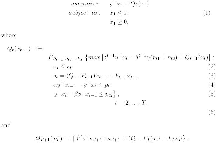
This model is based on the forest planning problem described by Ariyawansa and Felt in their collection of stochastic linear programming problems [AF05]. The goal is to maximize the value of timber, both cut and remaining, after the last period of planning. The constraints in this model pertain to the amount of forest cut in a single period, the age of trees, and the likelihood that trees remaining uncut are destroyed by fire.

Each tree belongs to one of K age classes of equal length. The length that defines the age classes is also used to define the length of stages of the planning period. Thus, trees belonging to age class A in a given stage will belong to age class A+1 in the next stage if they are not cut or destroyed by fire. Whenever any of these events take place, new trees are planted and, the number of trees in the first age class equals the sum of these two quantities.

The variables of the model are the total area of forest for each age class, for each period (vector s_t), the amount of forest harvested for each age class in each period (vector x_t), and penalty factors for not satisfying constraints on the amount of harvested area in each period (vectors p_t1 and p_t2).

A natural constraint is one that restricts the harvested area to be at most the total amount of area for each age class in each period t = 1,...,T:

x_t s_t

The next set of constraints on the harvested area involve penalty factors p_t1 and p_t2 which try to avoid the harvested quantities exceeding limits of how fast the timber industry can change its purchasing volume from the current period to the next:

y^Tx_t-1 - y^Tx_t p_t1
y^Tx_t-1 - y^Tx_t-1 p_t2

In these constraints and are constants and y is a vector representing the yield of selling one unit of harvested area of each class.

The matrices Q and P_t shown below are square matrices of dimension K that are used to express the total number of trees in each period for each age class, taking into account both harvesting and fire in the previous stage.

Thus, the following constraint expresses the total area in the beginning of period t, for t = 2,...,T:

s_t = (Q - P_t-1)x_t-1 + P_t-1x_t-1

Below, we describe the complete model.

In this model is a factor used to discount monetary values and depends on the inflation rate and the size of the planning period, v is a vector with the values of the trees in each age class, standing after the last period, and is a constant penalty factor. The objective function is to maximize the expected total profit.

The following table describes the constants, data, decision variables, and constraints of the model (with its corresponding names in the Mosel code).

Table 6.2: Model identifiers
Identifier Meaning

,,, (alpha,beta,gamma,delta) constants of the model (read from data file)

y (yield) yield of selling an unit of harvested area

v (v) value of the trees standing after the last period

x_t (x) amount of harvested forest of each age class in each period

s_t (s) total area of forest of each age class in each period

p_t1 (p1) penalty variable for not satisfying constraints YlowerLimit

p_t2 (p2) penalty variable for not satisfying constraints YUpperLimit

P matrix of sprands representing the probabilities of fire

ProbDiscret probability discretization of the realization of each fire probability

ValuesDiscret fire probability for each period

HarvestLimit constraints (1) and (2) in the model

Fix auxiliar constraint that fixes s₁ variables

s1 auxiliary data for fixing s₁ (initial planted area)

TotalArea constraints (3) in the model

YlowerLimit constraints (4) in the model

YupperLimit constraints (5) in the model

Below, we show the Mosel code that implements the model and solves it in Xpress-SP. The matrices Q and P_t are not stored explicitly as matrices. Instead, constraints (3) of the model are generated based on the structure of both matrices using the sprand P, as can be seen in the Mosel code for constraints TotalArea.
model forest_relax
 uses "mmsp"

 parameters
  EPS = 1e-5
 end-parameters
 
 declarations
  T=7
  K=8
  MAXDISCRET=3
  AGES = 1..K
  
  index:integer
  alpha,beta,delta,gama: real
  ScenariosAgg,ScenariosDel: set of integer
  yield, v: array (AGES) of real
  ProbDiscret,ValuesDiscret: array(1..MAXDISCRET, 1..MAXDISCRET) of real
  s1: array (AGES) of real
 end-declarations
 
 declarations
  P: array (AGES, 2..T+1) of sprand
  x: array (AGES, 1..T) of spvar
  s: array (AGES, 1..(T+1)) of spvar
  p1,p2: array (2..T) of spvar
  
  HarvestLimit: array (AGES, 1..T) of splinctr
  Fix: array (AGES) of splinctr
  TotalArea: array (AGES, 2..(T+1)) of splinctr
  YLowerLimit: array (2..T) of splinctr
  YUpperLimit: array (2..T) of splinctr
 end-declarations
 
! Read data
 initializations
 from 'forest.dat'
  yield
  v  alpha  beta  delta  gama
  ProbDiscret
  ValuesDiscret  s1
 end-initializations
 
! Create scenario tree
 declarations
  Stages = 1..(T+1)
  Branches: array (1..T) of integer
  Probabilities: array (1..MAXDISCRET) of real
  PValues: array (1..MAXDISCRET) of real
 end-declarations
 
 spsetstages(Stages)
 forall(t in 2..T+1, i in AGES) spsetstage(P(i,t), t)
 Branches:= [1, 3,3,3, 3,3,3]
 spcreatetree(Branches)
 
 forall(t in 2..T+1) do
  forall(i in 1..MAXDISCRET) PValues(i):= ValuesDiscret(Branches(t-1),i)
  forall(i in AGES) spsetrand(P(i,t), PValues)
 end-do
 
 forall(t in 1..T) do
  forall(i in 1..MAXDISCRET)
   Probabilities(i):= ProbDiscret(Branches(t),i)
  spsetprobcond(t+1,Probabilities)
 end-do
 
 setparam('xsp_scen_based', false)
 spgentree
 
! Objective function
 ObjFnc:= sum(t in 1..T, i in AGES) (delta^(t-1))*yield(i)*x(i,t) +
          sum(i in AGES)(delta^T)*v(i)*s(i,T+1) -
          gama*sum(t in 2..T) (delta^(t-1))*(p1(t) + p2(t))
! Spvars s(T+1) should be associated to stage T
 
! Constraints
 forall(j in AGES, t in 1..T) HarvestLimit(j,t):= x(j,t) <= s(j,t)
 forall(j in AGES) Fix(j):= s(j,1) = s1(j)
 
 forall(i in AGES, t in 2..(T+1))
  if i=1 then
   TotalArea(i,t):= s(i,t) = sum(j in AGES) (1 -P(j,t))*x(j,t-1) +
                    sum(j in AGES) P(j,t)*s(j,t-1)
  elif i=K then
   TotalArea(i,t):= s(i,t) = -(1-P(K-1,t))*x(K-1,t-1) -        
                    (1-P(K,t))*x(K,t-1) +
		    (1-P(K-1,t))*s(K-1,t-1) + 
		    (1-P(K,t))*s(K,t-1)
  else
   TotalArea(i,t):= s(i,t) = -(1 - P(i-1,t))*x(i-1,t-1) +  
                    (1 - P(i-1,t))*s(i-1,t-1)
  end-if
 
 forall(t in 2..T) do
  YUpperLimit(t):= - sum(j in AGES) yield(j)*x(j,t) + 
                   alpha*sum(j in AGES) yield(j)*x(j,t-1) <= p1(t)
  YLowerLimit(t):= sum(j in AGES) yield(j)*x(j,t) -  
                   beta*sum(j in AGES) yield(j)*x(j,t-1) <= p2(t)
 end-do
 
! Associate Spvars to stages
 forall(t in 1..T, i in AGES) do
  spsetstage(x(i,t),t)
  spsetstage(s(i,t),t)
 end-do
 forall(i in AGES) spsetstage(s(i,T+1),T)
 forall(t in 2..T) do
  spsetstage(p1(t),t)
  spsetstage(p2(t),t)
 end-do

 setparam('xsp_verbose', true)
 
! Optimize
 maximize(ObjFnc)
 
end-model
Note that an alternative structure of the scenario tree (different discretization) can be evaluated by changing the corresponding line of the Mosel code. For example, a tree with 3 branches at each stage may describe the problem more accurately and can be set by the statement Branches:= [1, 3,3,3, 3,3,3].

For the data we are using in the Appendix, the maximum number of branches (MAXDISCRET) in a node is 3. However, if the user provides the probabilities and the values of the corresponding sprand in the datafile, the branching structure can naturally be expanded to more than 3 branches.

Results

Running the model with the data provided in the Appendix gives the expected total profit of $4.23004e+007. This value is obtained for the problem when considering the structure of the scenario tree given by the statement Branches:= [1, 2,3,2, 2,2,2].

Analysis

The expected value version of the model has an optimal profit value of $4.21329e+007. The model is optimized with the following Mosel statement:
 maximize(ObjFnc, XSP_EV+XSP_REC) ! Expected value with recourse
The value of the stochastic solution is of the order

VSS = Z_R - Z_EVr = 1.675e+005

The perfect information version is solved by calling maximize as follows:
 maximize(ObjFnc, XSP_PI) ! Perfect information problem
This gives a profit of $4.51233e+007 and the value for the perfect information solution equal to

EVPI = Z_PI - Z_R = 2.8229e+006

In all three problems, the only nonzero first stage variable is x(1,8), that is associated to the last age class. Below, we show a table with the value of x(1,8) in the three problems:

Table 6.3: Stochastic problems
Problem Value of x(1,8) Objective Function

Recourse 20516.9 4.23004e+007

Expected value 20738.7 4.21329e+007

Perfect information 19770.3 4.51233e+007

Suppose that after solving the model the user wants to remove scenarios that give low values for the objective function. Below, we show an additional Mosel code that makes use of the routines speval and spdelscen to inspect the objective function value (profit) associated with each scenario. The scenarios where the objective function values are less than 95% of the optimal value for the stochastic problem are removed and the problem is solved again. Using this policy, the user iteratively removes scenarios until the objective function in all scenarios is greater than 95% of the new optimal objective function value.
Scenarios:= 1
 forall(t in 1..T) Scenarios *= Branches(t)

 while(true) do
  ScenariosDel:= {}
  forall(sce in 1..Scenarios| speval(ObjFnc,scen)<0.95*getobjval)
   ScenariosDel+= {scen}
  if (getsize(ScenariosDel)=0) then
   break
  end-if

  spdelscen(ScenariosDel)
  Scenarios -= getsize(ScenariosDel)

  maximize(ObjFnc)
  writeln(getobjval)
 end-do
The variable ScenariosDel is a set of integers that specifies the scenarios that will be deleted. The table below shows the objective function value for the stochastic problem at each iteration of this procedure, until there are no such scenarios to be removed.

Table 6.4: Expected profit after scenario deletion
Iteration Expected total profit

0 4.22529e+007

1 4.22907e+007

2 4.22990e+007

3 4.23034e+007

4 4.23041e+007

5 4.23072e+007

6 4.23096e+007

Iteration 0 refers to the objective function value of the original stochastic problem. The original problem had 729 scenarios and the final problem solved at iteration 6 had 675 scenarios. The scenario tree for this problem is generated by using the branching scheme Branches:= [1, 3,3,3, 3,3,3].

It is also possible to make a similar exercise, aggregating scenarios that have low probability by using the routines spgetscenprob and spaggregate. The following code aggregates scenarios that have probability less than 0.1% and are contiguous in the scenario tree, with the same parent node. After aggregation, we end up with 480 scenarios and expected total profit $4.2484e+007.
 Scenarios:= 1
 forall(t in 1..T) Scenarios *= Branches(t)
 
 ScenariosAgg:= {}
 forall(scen in 1..Scenarios | spgetprobscen(scen)<0.001)
  ScenariosAgg+= {scen}
 
 scen:= getsize(ScenariosAgg)
 AggOcurred:= false
 while(scen >= 1) do
  siblings:= {ScenariosAgg(scen)}
  forall(j in 1..(MAXDISCRET-1) | scen-j>0 ) do
   if (ceil(ScenariosAgg(scen-j)/Branches(T)) =
       ceil(ScenariosAgg(scen)/Branches(T))) then
    siblings+= {ScenariosAgg(scen-j)}
   else
    break
   end-if
  end-do

  if (getsize(siblings)>1) then
   writeln('aggregating ', siblings)
   spaggregate(siblings)
   AggOcurred:= true
  end-if
  Scenarios -= getsize(siblings) + 1
  scen -= getsize(siblings)
 end-do
 
 maximize(ObjFnc)
 writeln(getobjval)
The set ScenariosAgg is a set of integers that specifies the scenarios with probability less than 0.1%. From ScenariosAgg, we select the scenarios to be aggregated by checking if they have the same parent in stage 7. This task is done by using the information on the number of branches in stage 7:
 ceil(ScenariosAgg(scen)/Branches(T))
Below, we show a table that presents the differences between the node-based version and the scenario-based version of this model, in terms of number of rows and columns. The values are shown before and after pre-solving takes place, for the problem with 729 scenarios.

Before presolve After presolve

Rows Columns Rows Columns

Node Based 12400 8512 7922 5885

Scenario Based 183944 96228 4479 3758

Summary

In this section, we have just shown some of the features, embedded in Xpress-SP, that allow the user to optimize stochastic problems and perform further analysis in an easy and customizable way: by inspecting variables in particular scenarios, aggregating/deleting scenarios, obtaining estimates from the expected value and perfect information problems, and choosing among different ways of expanding the problem. These ideas play an important role in providing insight into the problem and simplifying or strengthening its formulation.

Assets and liabilities management for pension funds

Assets and liabilities management (ALM) problems are one of the most important classes of problems arising in the financial area. Typically the goal of these problems is to find an optimal strategy for allocating resources in order to obtain a profit that is sufficient to cover a certain type of liability. These problems often involve uncertain parameters; for instance, the returns received from different investments usually depend on unknown future market conditions. The amounts of liabilities that need to be paid at certain time can also depend on various future factors. Therefore, in many cases, applying stochastic programming techniques is crucial for making strategic decisions that efficiently handle the risk of possible losses.

We consider one of the practically important instances of these problems — assets and liabilities management for pension funds. A typical pension fund has members that can be separated into two classes. The first class is `active members', i.e., employees paying a certain fraction of their wages to the pension fund each month. The second class is `non-active' members, i.e., people who have retired and receive payments from the pension fund. At every time period the pension fund should have enough assets to be able to cover all the payments (liabilities). The problem the pension fund manager is faced with is minimizing the contribution rate (fraction of wages) paid by the active members while being able to cover the liabilities. The setup of the problem aims to ensure that the percentage of wages that the employees pay is small enough to attract new pension fund members. To cover the liabilities, assets owned by the fund are invested into stocks, whose returns are uncertain. Moreover, the amount of liabilities is also uncertain, since it depends on the inflation rate and demographic factors. Stochastic programming techniques allow one to expand the deterministic formulation of the model by using scenario data for uncertain parameters.

First, we present the formal setup of the model. These are its parameters, decision variables, and the deterministic formulation (assuming that all the parameters are known and no uncertainty is involved). Here we consider the one-period model, i.e., there is only one planning period, where the investment decision is made at the initial moment in order to cover the liabilities at the end of the period.

Parameters of the model

A₀ – the initial value of all assets owned by the fund.
W₀ – the total amount of wages of the active members at the initial moment.
l₀ – the payments made by the fund at the initial moment.
r_n– the rate of return of the stock number n, n = 1, ..., N.
L – the liability measure that should be exceeded by the total value of assets at the end of the period.
– the parameter used to control the behavior of the fund. We want the total return to exceed the liabilities by a certain amount, for instance, if = 1.3 then we want the total return to be at least 30% higher than the liabilities.

Decision variables

x_n – the total amount of money invested in the stock number n, n = 1, ..., N.
y – the contribution rate (fraction of wages) that is added to the initial assets at the initial time moment.

Deterministic problem formulation

Z=min_{y R, x R^N}y

^N

_n=1_n

=A₀-l₀+W₀y

^N

_n=1_n_n

L

x_n0 n {1..N}

Description

The first constraint is the investment balance: the total money invested in the stocks x_n should be equal to the total assets available at the beginning of he period, i.e., the initial assets plus the fraction of wages paid by active members minus payments made at the beginning of the period.

The second constraint expresses the fact that the total return at the end of the period must exceed the amount of liabilities (multiplied by the control parameter ).

The third set of constraints is the non-negativity constraints on x_n that means that we don't allow any `short' positions or borrowing. Note that we don't impose any restrictions on y, we allow it to be negative. If y is negative, it means that the fund can cover all the liabilities without taking money from active members and even make additional payments to them.

Stochastic problem formulation

We now consider the ALM problem with N = 12 stocks and S = 5000 scenarios corresponding to the realizations of the returns and liabilities. We create the scenario tree based on the real-life data representing returns of 12 stocks, as well as the amount of liabilities. This tree has two stages and 5000 nodes at the second stage. Certain realizations of the returns and liabilities correspond to each node at the second stage. The probabilities of all realizations are assumed to be the same and equal to P = 1/S.

The extended two-stage formulation of the problem can be written as follows:

Z=min_{y R, x R^N}y

^N

_n=1_n

=A₀-l₀+W₀y

^N^s

_n=1_n_n

L^s s {1..S}

x_n0 n {1..N}

Mosel implementation

Using stochastic modeling tools in Mosel, one can create the scenario tree representing stochastic parameters of the model and specify the constraints of the deterministic model then the extended (stochastic) problem formulation is generated automatically. The Mosel implementation of the stochastic model is presented below.
model ALM_sp
 uses 'mmsp'                ! Use the stochastic programming module
 
 parameters
  psi=1.3 
 end-parameters
 
 declarations
  Stocks=1..12              ! Set of stocks
  Intial_Asset,A: real
  Initial_payment,l: real   ! Payments at the initial time
  Total_wages,W: real       ! Total amount of wages of active members
                            ! of the fund
 end-declarations
 
! Initial (deterministic) parameters
 initializations from 'ALM.dat'
  Intial_Asset Initial_payment Total_wages
 end-initializations
 
 A:=1                             ! Scaled value of initial assets
 l:=Initial_payment/Intial_Asset  ! Scaled value of initial payments
 W:=Total_wages/Intial_Asset      ! Scaled value of wages
 
 
 declarations
  Stages = {"First","Second"}     ! Two stages - one-period model 
! Random parameters
  return: array(Stocks) of sprand ! Uncertain returns of the stocks
  L: sprand                       ! Uncertain liabilities  
! Decision variables
  x: array(Stocks) of spvar       ! Amount invested into each stock
  y: spvar                        ! % of wages paid by active members
! Model objective and constraints
  fraction: splinctr
  inv_balance: splinctr
  minreturn: splinctr
 end-declarations
 
! Allow contribution rate to be both positive and negative
 y is_free 
  
! Setting stages
 spsetstages(Stages)
 forall(p in Stocks) spsetstage(return(p),"Second")
  spsetstage(L,"Second")
 
! Scenarios declaration and generating scenario tree
 declarations
  S = 500
  Scen = 1..S
  Values: array(Scen, Stocks) of real
  Liab: array(Scen) of real
 end-declarations

 spcreatetree(S)
 forall(s in Scen) prob(s):=1/S
 spsetprobcond(2,prob)
 
 initializations from 'returns.dat'
  Values
 end-initializations
 
 initializations from 'Liabilities.dat'
  Liab
 end-initializations
 
 forall(p in Stocks,s in Scen) spsetrandatnode(return(p),s,Values(s,p))
 forall(s in Scen) spsetrandatnode(L,s,Liab(s)/Intial_Asset)
 spgentree
  
! Model definition 
 fraction:= y
 inv_balance:=sum(p in Stocks)1*x(p) = A - l + W*y
 minreturn:=sum(p in Stocks)(1+return(p))*x(p) >= psi*L
 
! Assigning variables to stages
 forall(p in Stocks) spsetstage(x(p),"First")
 spsetstage(y,"First") 
 
! Optimizing
 minimize(fraction)
 
! Solution output
 writeln("psi = ", psi)
 writeln("contribution rate = ", getobjval)
 forall(p in Stocks) writeln("x(", p, ") = ", getsol(x(p)))
  
 end-model
Note that for convenience the monetary parameters of the model are scaled, i.e., divided by the amount of the initial assets A₀. The description of the data files data.dat and data_L.dat used for generating the scenario tree can be found in the Appendix. The expected value (Z_EV) and perfect information (Z_PI) solutions can be found by running this program after modifying the line minimize(fraction) by minimize(fraction,XSP_EV) and minimize(fraction,XSP_PI) respectively.

Analysis of the results

Table Optimal objective values for different values of . (see Appendix) presents the values of the objective function (i.e., contribution rate) for the original stochastic problem (Z*), and for the expected value and perfect information problems, for different values of the control parameter . The differences between these solutions are also calculated.

An interesting observation is that all these solutions, as well as the differences Z*- Z_EV and Z*- Z_PI are linear functions of (see Figure Linear dependency of the optimal solutions ). Linear dependency of Z*, Z_EV and Z_PIof can be easily proven theoretically, using LP sensitivity analysis techniques. Since Z*, Z_EV and Z_PIare linear functions of , the differences Z*- Z_EV and Z*- Z_PI representing the `value' of deterministic solution and perfect information are also linear with respect to . Note that the optimal stochastic solution is much larger than the corresponding expected value and perfect information solutions, which means that one is forced to take more conservative decisions (i.e., spend more money) if uncertainty is taken into account. Also, as increases, the values Z*- Z_EV and Z*- Z_PI also increase, which means that the stochastic solution becomes more `expensive' if a greater amount of liabilities needs to be covered.

Figure 6.12: Linear dependency of the optimal solutions w.r.t. .

It is also important to look at the optimal investment strategy found from solving the stochastic problem. As one can see from Table Investment decisions (scaled values) for different values of . (see Appendix), the relative structure of the investments remains the same for all considered 's, however, the amounts invested into each stock increase as increases.

Another issue that we address here is how the structure of the scenario dataset affects the optimal solution of the stochastic problem. For this purpose, we calculated the mean _n and the standard deviation _n of the return of each considered stock, over 5000 scenarios. Then we delete all scenarios where the value of the return of at least one stock lies outside the interval [_n -m_n , _n + m_n], for some value of m. This procedure allows one to reduce the variability of the scenarios by excluding `extreme' values of the returns, which can be both positive and negative. Deletion of a set of scenarios can be performed using the function spdelscen(). By changing the parameter m, we control the length of the interval and establish the bounds for possible values of the returns. The purpose of this procedure is to compare the solution of the initial problem and the solutions corresponding to the problems with fewer scenarios having smaller variability.

As one can intuitively predict, the optimal solution will be `cheaper' if the length of this interval is small, and the contribution rate will increase as the interval length grows, since the minimum return constraint needs to be satisfied for all scenarios, including realizations with extreme unfavorable returns. As a limiting case, when m is large enough to include all the considered set of scenarios, the solution of the original stochastic problem is obtained. These results are summarized in Table 8.

Figure 6.13: Optimal solutions of the stochastic problem for different sets of scenarios.

Figure Optimal solutions of the stochastic problem for different sets of scenarios. shows the plot of the optimal solution value with respect to the number of scenarios considered. As one can see, when the number of scenarios is very close to 5000, the optimal solution is almost the same as the `true' solution corresponding to the problem with all 5000 scenarios; however, as the number of scenarios decreases, the optimal objective value drops down. This happens because the `extreme' scenarios that affect the solution are deleted from the scenario tree, resulting in a less expensive solution. The difference between the true solution and the solution obtained after the deletion of scenarios remains relatively small as long as the number of remaining scenarios is large enough (2000). This sufficiently reflects the variability of the returns; however, this difference rapidly increases if more scenarios are deleted. In fact, if we leave only the scenarios where all the returns lie in the interval [_n -_n , _n + _n], the optimal solution value is almost twice smaller than in the case of the full set of 5000 scenarios. These facts show that the appropriate choice of the scenarios dataset is important for obtaining the solution of the stochastic problem that would properly reflect the uncertainty.

Assemble to order system

Refer to Section 5 in the paper [DVNT05].

Options contract in supply chains

Refer to Section 6 in the paper [DVNT05]

Power management in a hydro-thermal system

Stochastic Programming has been used extensively in the energy sector for various purposes such as planning of capacity expansion, unit commitment, making pricing decision in the electricity market, etc. The following example has been inspired from the work of Gröwe-Kuska et al. (see [GKNR02]). Here we consider a hydro-thermal system in which hourly decisions pertaining to operational levels of the units need to be made under uncertain demand load.

Description

There are T time periods. I and J are the numbers of thermal and hydro units, respectively. For a thermal unit i in period t, u_i,t {0,1} is its commitment (1 if on, 0 if off) and p_i,t its production, with p_i,t = 0 if u_i,t= 0, p_i,t [P_i,t^min, P_i,t^max] if u_i,t = 1. Additionally there are minimum up/down-time requirements: when unit i is switched on (off) it must remain on (off) for at least _i^up (_i^dn) periods. For a hydro plant j, s_j,t and w_j,t are its generation and pumping levels in period t with upper bounds S_j,t^max and W_j,t^max respectively, and l_j,t is the storage volume in the upper dam at the end of period t with upper bound L_j,t^max. The water balance relates l_j,t with l_j,t-1, s_j,t, w_j,t and water inflow _j,t using the pumping efficiency _j. The initial and final volumes are specified by l_jⁱⁿ and l_j^end.

The basic system requirement is to meet the electric load. Another important requirement is the spinning reserve constraint. To maintain reliability (compensate sudden load peaks or unforeseen outages of units) the total committed capacity should exceed the load in every period by a certain amount (e.g., a fraction of the demand). The load and the spinning reserve during period t are denoted by d_t and r_t, respectively.

Efficient operation of pumped storage hydro plants exploits daily cycles of load curves by generating during peak load periods and pumping during off-peak periods. Since the operating costs of hydro plants are usually negligible, the total system cost is given by the sum of startup and operating costs of all thermal units over the whole scheduling horizon. The fuel cost C_i,t for operating thermal unit i during period t has the form
C_i,t = max _{l {1..L}} {a_i,l,t·p_i,t + b_i,l,t·u_i,t}
The startup cost of unit i depends on its downtime; it may vary from a maximum cold start value to a much smaller value when the unit is still relatively close to its operating temperature. This is modeled by the startup cost
S_i,t = max _{{1..^c_i}} {u_i,t-_{k {1..}}u_i,k-}
where 0 = c_i,0 < ... < c_{i_i^c} are fixed cost coefficients. _i^c is the cool-down time of unit i, c_{i_i^c} is its maximum cold-start cost, u_i, {ⁱⁿⁱ,...,0} are given initial values, where ⁱⁿⁱ = max_i{1,...,I}{_i^c, 1-_i^up, _i^dn-1}.

Model

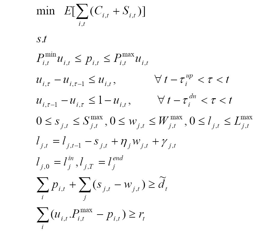
Uncertainty

The uncertainty in the model—demand in each period—is dealt with as follows:

We begin by aggregation of periods. As the number of periods increases, the possibilities of realization of demand increase exponentially. From the stochastic optimization point of view, some of the consecutive periods may be aggregated together to form a stage, e.g., periods {1,...,t₁} may be set to stage 1, periods {t₁+1,...,t₂} to stage 2,..., and periods {t_K+1,...,T} to stage N as shown in the following Figure Aggregated stages.

Figure 6.14: Aggregated stages

Demand, being random, may be identified based on a time series or regression model. Here we simply assume the demand process to be d˜_t = _t + ˜_td˜_t-1 + ˜_t, where , , are given, and ˜_t Uniform(^min,^max), and ˜_t Normal(0,1)

Based on the demand process, we determine an initial structure of the scenario tree. We compute values of demands in various scenarios using the sample means and standard deviations of the simulated scenarios by running M simulations. If d_t^m is the value of demand in the m^th run then estimated

mean demand: _t=

^M^m

_m=1_t

M

, and

variance in demand: ²_t=

^M^m²

_m=1_t_t

M-1

Next, we build a stable and small scenario tree using the estimates and aggregated stages as follows:

Re-model the demand process as
d_t=_t+

^t^1/2

_t'=2_Stg(t')

, where Stg(t) is the aggregated stage where period t belongs to, and ˜₂, ...,˜_N {1 w.p 0.5, -1 w.p 0.5}

Generate an exhaustive binary tree based on possible realizations of ˜₂, ..., ˜_N as shown below.

Figure 6.15: Binary scenario tree with 2^N-1 scenarios

As the number of aggregated stages increase, the number of scenarios may increase rapidly, therefore we may reduce the scenario tree using the following schema.

Define the distance between vectors vⁱ and v^j as c^h(vⁱ,v^j) = max{1, vⁱ^h-1, v^j^h-1}·vⁱ-v^j where h is a given parameter, and . is a Euclidian norm.

Let realizations of ˜ = [˜₂, ..., ˜_N] in scenario k be vector ^k. Given S scenarios with probabilities P₁,...,P_S, we delete a scenario k = argmin_l{1,...,S}{P_l, min_{s{1,...,S}:sl} c^h(^l,^s)}. Then, roughly speaking, deletion of a scenario k occurs when it is close to another scenario s as measured by the distance or where its probability is small. The reduced scenario tree has one less scenario; scenario k is deleted, and P_s is incremented by P_k. This step is repeated until the final number of scenarios reaches a prescribed number S' that is reasonably small to represent the uncertainty, and would yield sufficiently accurate solution to the problem.

Next, we decouple S' scenarios by:

Creating a scenario tree with S' branches from the node in the 1^st stage, and 1 branch per node from each node in other stages.

Setting the realized values of ˜, and revised probabilities of scenarios. The scenario tree would look as shown in the following Figure Reduced scenario tree with S' scenarios.

Figure 6.16: Reduced scenario tree with S' scenarios

Many realizations of ˜'s until certain stages are the same, hence we restructure the reduced scenario tree by clubbing together all the realizations that are equal as follows:

Define node_t,n for the n^th node in the t^th stage of the scenario tree. Let PossScen_t,n be set of scenarios that branches off from node_t,n that have same realized values of ˜_t+1

Find all such possible sets of the PossScen_t,n's corresponding to the realizations of ˜_t+1

Each of the set PossScen_t,n forms a new child of node_t,n with the conditional probability: _{sPossScen_t,n}P_s / P_t,n, where P_t,n is the unconditional probability of occurrence of node_t,n. While keeping track of number of children of node_t,n, number of nodes in stage t, and unconditional probability P_t,n of node_t,n, incrementally build a scenario tree. The re-structured scenario tree would look as follows.

Figure 6.17: Re-structured scenario tree with S' scenarios

Optimization

The optimization model is built in Xpress-SP by associating all decision variables in period t to Stg(t). The scenario tree is built by running simulation, building a binary scenario tree, and reducing it by deleting few scenarios as described in previous section. The model excerpt is shown below.
 declarations
  p,S,C: array(ThermalUnits,TimeBlocks) of spvar
  u: array(ThermalUnits,(tau_ini..0)+TimeBlocks) of spvar
  s,w,l: array(HydroUnits,TimeBlocks) of spvar
  lam: array(ThermalUnits,TimeBlocks,1..L) of spvar
  
  TotalCost: splinctr
  UBprod: array(ThermalUnits,TimeBlocks) of splinctr
  LBprod: array(ThermalUnits,TimeBlocks) of splinctr
  UBstoreageBal: array(HydroUnits,TimeBlocks) of splinctr
  Minuptime,Mindowntime: dynamic array(ThermalUnits,range,TimeBlocks) of splinctr
  Load: array(TimeBlocks) of splinctr
  SpinningReserve: array(TimeBlocks) of splinctr
  ProdLevel,FuelCost,SumToOne: array(ThermalUnits,TimeBlocks)  of splinctr
  Prodtn: dynamic array(ThermalUnits,TimeBlocks) of splinctr
  StartupCost: array(ThermalUnits,range,TimeBlocks) of splinctr
 end-declarations

 forall(i in ThermalUnits, t in (tau_ini..0)+TimeBlocks) u(i,t) is_binary
  
 forall(t in tau_ini..0,i in ThermalUnits) do
  spsetstage(u(i,t),1)
  u(i,t)=0
 end-do
   
 forall(i in ThermalUnits,t in TimeBlocks)
  UBprod(i,t):=p(i,t)<=P_max(i)*u(i,t) 
 forall(i in ThermalUnits,t in TimeBlocks)
  LBprod(i,t):=p(i,t)>=P_min(i)*u(i,t)
 forall(j in HydroUnits,t in TimeBlocks)
  s(j,t)<=S_max(j)
  
 forall(j in HydroUnits,t in TimeBlocks)
  w(j,t)<=W_max(j)
 forall(j in HydroUnits,t in TimeBlocks)
  l(j,t)<=SL_max(j)
 forall(j in HydroUnits,t in TimeBlocks)
  if t=1 then
   UBstoreageBal(j,t):= l(j,t)=l_in(j)-s(j,t)+eta(j)*w(j,t)+gamma(j,t)
  elif t=T then
   UBstoreageBal(j,t):= l_end(j)=l(j,t-1)-s(j,t)+eta(j)*w(j,t)+gamma(j,t)
  else
   UBstoreageBal(j,t):= l(j,t)=l(j,t-1)-s(j,t)+eta(j)*w(j,t)+gamma(j,t)
  end-if

 forall(i in ThermalUnits, t in TimeBlocks, tau in (t-tau_up(i)+1)..(t-1) | 
   t-tau_up(i)+1<=t-1 and tau-1>=tau_ini)
   Minuptime(i,tau,t):=u(i,tau)-u(i,tau-1)<=u(i,t)
 forall(i in ThermalUnits, t in TimeBlocks, tau in (t-tau_dn(i)+1)..(t-1) | 
   t-tau_dn(i)+1<=t-1 and tau-1>=tau_ini)
   Mindowntime(i,tau,t):=u(i,tau-1)-u(i,tau)<=1-u(i,t)
  
 forall(t in TimeBlocks) 
  Load(t):=sum(i in ThermalUnits) p(i,t)+
           sum(j in HydroUnits) (s(j,t)-w(j,t))>=d(t)

 forall(t in TimeBlocks) SpinningReserve(t):=
  sum(i in ThermalUnits) (P_max(i)*u(i,t)-p(i,t))>=r(t)

 forall(i in ThermalUnits, t in TimeBlocks) do
  ProdLevel(i,t):=p(i,t)=
   sum(l_ in 1..L) prodt(i,t,l_)*lam(i,t,l_)

  FuelCost(i,t):=C(i,t)=sum(l_ in 1..L) cost(i,t,l_)*lam(i,t,l_)
  
  SumToOne(i,t):=sum(l_ in 1..L) lam(i,t,l_)=u(i,t)
   Prodtn(i,t):=sum(l_ in 1..L) prodt(i,t,l_)*lam(i,t,l_)
   Prodtn(i,t) is_sos2
 end-do

 forall(i in ThermalUnits,t in TimeBlocks,tau in 0..tau_c(i))
  StartupCost(i,tau,t):=
   S(i,t)>=c(i,tau)*(u(i,t)-sum(k in 1..tau) u(i,t-k))

 TotalCost:=sum(i in ThermalUnits,t in TimeBlocks) (C(i,t)+S(i,t))
Implementation

The model is implemented for 24 time periods (1 day) aggregated into 5 stages, 2 hydro units and 3 thermal units. A visual interface is built to visualize the demand and optimal solutions in various scenarios as shown in the following figure.

Figure 6.18: Interface for visualization of hydro-thermal generation under uncertain load

[Next] [Index]

If you have any comments or suggestions about these pages, please send mail to docs@dashoptimization.com.

Products	Destinations	SellingPrice	CostOfLostSales	CostOfExcessSales
Shirts	NYC	25	0.75	10
Shirts	LA	20	0.25	8
Trousers	NYC	45	1.5	15
Trousers	LA	40	0.5	15

Identifier	Meaning
a_ij (A)	number of hours required by aircraft of type i to complete a flight of route j
a_ijk (Aswitch)	as the number of hours required by aircraft of type i to fly route k after having been switched from route j
x_ij (x)	number of flights planned for route j using aircraft of type i
x_ijk (xswitch)	increase of flights in route k after switching aircraft i from route j
F_i (F)	maximum number of flight hours for aircraft of type i during a month
c_ij (Cost)	cost of initially assigning aircraft of type i to fly one flight of route j
c_ijk (CostSwitch)	cost for aircraft of type i to fly one flight of route k after having been switched from route j
c_j⁺ (cplus)	cost of transporting one unit of demand of route j by a commercially contracted flight
c_j^- (cminus)	cost of one unit of unused capacity on route j
y_j⁺ (yplus)	demand of route j commercially contracted in the recourse
y_j^- (yminus)	unused capacity assigned to route j
b_ij (b)	carrying capacity of aircraft of type i when flying in route j
d_j (d)	demand of route j
MaxHours(i)	constraints (1) of the model
MaxSwitch(i,j)	constraints (2) of the model
DemandCtr(j)	constraints (3) of the model
ExpTotalCost	objective function

Identifier	Meaning
,,, (alpha,beta,gamma,delta)	constants of the model (read from data file)
y (yield)	yield of selling an unit of harvested area
v (v)	value of the trees standing after the last period
x_t (x)	amount of harvested forest of each age class in each period
s_t (s)	total area of forest of each age class in each period
p_t1 (p1)	penalty variable for not satisfying constraints YlowerLimit
p_t2 (p2)	penalty variable for not satisfying constraints YUpperLimit
P	matrix of sprands representing the probabilities of fire
ProbDiscret	probability discretization of the realization of each fire probability
ValuesDiscret	fire probability for each period
HarvestLimit	constraints (1) and (2) in the model
Fix	auxiliar constraint that fixes s₁ variables
s1	auxiliary data for fixing s₁ (initial planted area)
TotalArea	constraints (3) in the model
YlowerLimit	constraints (4) in the model
YupperLimit	constraints (5) in the model

Problem	Value of x(1,8)	Objective Function
Recourse	20516.9	4.23004e+007
Expected value	20738.7	4.21329e+007
Perfect information	19770.3	4.51233e+007

Iteration	Expected total profit
0	4.22529e+007
1	4.22907e+007
2	4.22990e+007
3	4.23034e+007
4	4.23041e+007
5	4.23072e+007
6	4.23096e+007

	Rows	Columns	Rows	Columns
	Before presolve		After presolve
Node Based	12400	8512	7922	5885
Scenario Based	183944	96228	4479	3758